Summary of the Previous Session
In our last session, we introduced the Multiphase Optimization Strategy (MOST) and explored how it differs from traditional randomized controlled trials (RCTs). While RCTs evaluate an intervention as a whole, MOST focuses on optimizing individual components before assembling the final intervention package. Using the example of a stress-reduction app for college students, we identified its three key components—mindfulness exercises, physical activity goals, and social support features—and examined their individual effects, costs, and interactions. We also introduced the four guiding principles of intervention optimization: Effectiveness, Affordability, Scalability, and Efficiency (EASE).
In today’s session, we will focus on how to implement MOST principles in practice. Continuing with the stress-reduction app example, we will design an experiment to systematically test different combinations of intervention components, apply factorial design as a tool to analyze their effects, and determine the most effective, efficient, and scalable intervention. By the end of this session, we will have a clear understanding of how to use MOST to guide intervention development and optimization before moving to full-scale evaluation. Let’s get started!
Implementing MOST for the Stress-Reduction App
This example demonstrates how to apply the Multiphase Optimization Strategy (MOST) to develop and refine an intervention aimed at reducing stress among college students. The intervention comprises three components:
Mindfulness Exercises – Cost: $15 per participant Teaches meditation and breathing techniques to regulate emotions and reduce stress.
Physical Activity Goals – Cost: $30 per participant Uses endorphin release and improved well-being through regular exercise to lower stress.
Social Support Systems – Cost: $25 per participant Builds relationships and reduces isolation, which in turn buffers stress.
Preparation Phase
The Preparation Phase establishes the intervention’s theoretical framework, components, and specific optimization objectives.
A. Conceptual Model
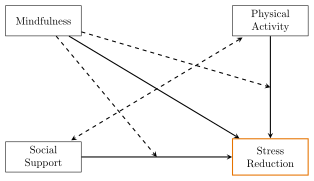
Each component addresses stress via distinct mechanisms:
Mindfulness: Reduces acute stress responses.
Physical Activity: Improves long-term resilience and mood.
Social Support: Mitigates feelings of isolation and fosters peer encouragement.
B. Optimization Objective
We aim to maximize stress reduction while keeping the per-participant cost at or below $50. Including all three components would cost $70 ($15 + $30 + $25), so we must determine the most cost-effective combination.
C. Hypotheses
Mindfulness alone may yield moderate stress reduction, but combining it with Physical Activity or Social Support could enhance effectiveness.
Physical Activity and Social Support may have interactive effects, possibly increasing motivation and adherence.
There may be diminishing returns when adding multiple components, requiring careful cost-effectiveness analysis.
Optimization Phase
In this phase, we conduct an optimization trial to identify the combination of components that best meets the targeted constraints and outcomes.
A. Experimental Design
A 222 factorial design efficiently evaluates multiple components and their potential interactions. Each of the three components (Mindfulness, Physical Activity, Social Support) can be either included (Yes) or excluded (No), resulting in eight experimental conditions:
| Group | Mindfulness | Physical Activity | Social Support | Total Cost |
|---|---|---|---|---|
| 1 | Yes | Yes | Yes | $70 (Over budget) |
| 2 | Yes | Yes | No | $45 |
| 3 | Yes | No | Yes | $40 |
| 4 | Yes | No | No | $15 |
| 5 | No | Yes | Yes | $55 (Over budget) |
| 6 | No | Yes | No | $30 |
| 7 | No | No | Yes | $25 |
| 8 | No | No | No | $0 (Control) |
B. Determine the Requiered Sample Size
To determine the required sample size per group, we follow standard power analysis procedures for factorial designs. The key factors that influence the sample size calculation are:
Significance Level ()
The probability of making a Type I error (false positive).
Standard choice: .Statistical Power ()
The probability of correctly detecting an effect if it exists.
Standard choice: (80%) or (90%) for higher confidence.Expected Effect Size ( or )
The magnitude of the effect you expect to observe.Small:
Medium:
Large: (Cohen, 1988)
Since this is a behavioral intervention, a small to medium effect size ( to ) is common.
Number of Factors and Levels
The design consists of 3 factors, each with 2 levels (Yes/No):
The total sample size () for a factorial ANOVA is calculated using: where:
is the noncentrality parameter (NCP)
is the effect size (Cohen’s )
We aim to calculate the required sample size for a factorial ANOVA with three factors, each having two levels, assuming:
Significance level:
Power:
Effect size (Cohen’s ):
Number of groups:
Step 1: Compute Degrees of Freedom
The degrees of freedom for the between-group effect is:
The within-group degrees of freedom () depends on the total sample size and is initially approximated as a large number (e.g., ) for estimating the critical F-value.
Step 2: Compute the Critical F-Value
The critical F-value is determined from an F-distribution table at : Using statistical functions, we obtain:
data f_critical;
    alpha = 0.05;  /* Significance level */
    df1 = 7;       /* Degrees of freedom for the numerator */
    df2 = 10000;   /* Degrees of freedom for the denominator (large sample approximation) */
    f_crit = quantile("F", 1 - alpha, df1, df2);
    put f_crit=;
run;
Listing 5.1. SAS Code to Compute Critical F-Value
Step 3: Compute the Noncentrality Parameter (NCP)
The noncentrality parameter () is given by: Substituting the values:
Step 4: Compute Total Sample Size
The total sample size () is calculated using: Substituting the values: Thus, the total sample size required is approximately:
Step 5: Compute Sample Size Per Group
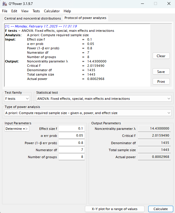
The sample size per group is given by: Thus, each group should have approximately 176 participants. To compute the sample size using G*Power, follow these steps:
Open G*Power software.
Select "F tests" as the test family.
Choose "ANOVA: Fixed effects, special, main effects and interactions" as the statistical test.
In the "Type of power analysis" dropdown, select "A priori: Compute required sample size – given , power, and effect size".
Set the effect size () to 0.1.
Set (Significance level) to 0.05.
Set the desired power level to 0.8.
Set the number of groups to 8 (since it is a factorial design).
Set degrees of freedom to 7.
Click "Calculate" to obtain the total sample size.
Data Collection & Analysis
Through random assignment, ensure each participant is placed into one of the eight conditions described in Table 5.1. The Primary Outcome is stress reduction (measured by self-report scales, physiological markers, etc.). Secondary Outcome includes metrics like engagement (frequency of app use) and adherence (how consistently participants follow the intervention).
This SAS code generates synthetic data for a factorial design study of a stress-reduction app, where the three factors (Mindfulness, Physical Activity, Social Support) each have two levels ("Yes"/"No") resulting in 8 unique experimental conditions. For each condition, 176 observations are simulated, yielding a total of 1,408 subjects. The code assigns binary factor levels based on the group index, computes a cell-specific mean response (starting from a baseline of 50 and adjusting for main effects—reductions of 5, 3, and 2 units for Mindfulness, Physical Activity, and Social Support respectively—and an additional interaction effect when both Mindfulness and Social Support are "Yes"), and then generates an individual response by adding normally distributed random error (with a standard deviation of 10). This dataset can be used for subsequent factorial analysis.
data synthetic;
   call streaminit(123); /* Set random seed for reproducibility */
   do group = 1 to 8;  /* 8 groups (cells) */
      do i = 1 to 176; /* 176 observations per group */
         /* For group 1 to 8, we determine factor levels by treating group-1 as a binary index (0 to 7) */
         b = group - 1;
         /* Convert b into binary digits for 3 factors:
            - The most significant bit for Mindfulness,
            - The next for Physical Activity,
            - The least for Social Support.
         */
         Mindfulness = ifc(mod(floor(b/4),2)=1, "Yes", "No");
         PhysicalActivity = ifc(mod(floor(b/2),2)=1, "Yes", "No");
         SocialSupport = ifc(mod(b,2)=1, "Yes", "No");

         /* Compute the cell-specific mean response */
         meanY = 50;  /* baseline stress level */
         if Mindfulness = "Yes" then meanY = meanY - 5;
         if PhysicalActivity = "Yes" then meanY = meanY - 3;
         if SocialSupport = "Yes" then meanY = meanY - 2;
         /* Example interaction: if both Mindfulness and SocialSupport are "Yes", further reduce by 1 unit */
         if Mindfulness = "Yes" and SocialSupport = "Yes" then meanY = meanY - 1;

         /* Generate the observed response with error variance = 10^2 */
         Response = meanY + rand("normal", 0, 10);

         output;
      end;
   end;
   drop group i b;
run;
Listing 5.2. SAS Code to Generate Synthetic Data
This SAS code performs a factorial ANOVA using PROC GLM on the synthetic dataset for our stress-reduction app study. The CLASS statement defines the three categorical factors—Mindfulness, Physical Activity, and Social Support—while the MODEL statement specifies the full factorial model including all main effects, two-way interactions, and the three-way interaction. Least-squares means are computed with Tukey’s adjustment for multiple comparisons, and contrast statements are used to test the specific hypotheses for each main effect. This analysis is consistent with the Multiphase Optimization Strategy (MOST) approach to evaluating intervention components.
proc glm data=synthetic;
   class Mindfulness (ref="No") PhysicalActivity (ref="No") SocialSupport (ref="No") ;
   model Response = Mindfulness PhysicalActivity SocialSupport
                    Mindfulness*PhysicalActivity
                    Mindfulness*SocialSupport
                    PhysicalActivity*SocialSupport
                    Mindfulness*PhysicalActivity*SocialSupport / solution;
   /* Get overall tests of significance for the model */
   lsmeans Mindfulness PhysicalActivity SocialSupport / adjust=tukey;
   /* Optionally, request tests for interactions */
   contrast 'Mindfulness main effect' Mindfulness 1 -1;
   contrast 'Physical Activity main effect' PhysicalActivity 1 -1;
   contrast 'Social Support main effect' SocialSupport 1 -1;
   run;
quit;
Listing 5.3. SAS Code to Perform Factorial Analyis
This code generates the following output.
| Source | DF | Sum of Squares | Mean Square | F Value | Pr F |
|---|---|---|---|---|---|
| Model | 7 | 19631.55 | 2804.51 | 27.12 | 0.0001 |
| Error | 1400 | 144758.15 | 103.40 | ||
| Corrected Total | 1407 | 164389.70 |
| Source | DF | Type I SS | Mean Square | F Value | Pr F |
|---|---|---|---|---|---|
| Mindfulness | 1 | 13777.42 | 13777.42 | 133.25 | 0.0001 |
| PhysicalActivity | 1 | 2127.80 | 2127.80 | 20.58 | 0.0001 |
| SocialSupport | 1 | 3341.93 | 3341.93 | 32.32 | 0.0001 |
| Mindfulne*PhysicalAc | 1 | 12.23 | 12.23 | 0.12 | 0.7309 |
| Mindfulne*SocialSupp | 1 | 291.93 | 291.93 | 2.82 | 0.0931 |
| PhysicalA*SocialSupp | 1 | 24.93 | 24.93 | 0.24 | 0.6235 |
| Mindfu*Physic*Social | 1 | 55.29 | 55.29 | 0.53 | 0.4647 |
| Parameter | Estimate | Standard Error | t Value | Pr |
|---|---|---|---|---|
| Intercept | 50.93 | 0.77 | 66.45 | |
| Mindfulness | -5.93 | 1.08 | -5.47 | |
| PhysicalActivity | -3.31 | 1.08 | -3.05 | 0.0023 |
| SocialSupport | -2.83 | 1.08 | -2.61 | 0.0091 |
| Mindfulne*PhysicalAc | 1.17 | 1.53 | 0.76 | 0.4472 |
| Mindfulne*SocialSupp | -1.03 | 1.53 | -0.67 | 0.5023 |
| PhysicalA*SocialSupp | 1.32 | 1.53 | 0.86 | 0.3876 |
| Mindfu*Physic*Social | -1.59 | 2.17 | -0.73 | 0.4647 |
Based on the GLM output, the overall model is highly significant , indicating that the combination of intervention components explains a significant portion of the variance in stress reduction (). Each main effect is robustly significant: Mindfulness , Physical Activity , and Social Support all contribute independently to reducing stress. Notably, the interaction between Mindfulness and Social Support shows partial significance at our threshold, suggesting that when these components are combined, they may have an additional modest effect on stress reduction beyond their individual contributions. In contrast, the interactions between Mindfulness and Physical Activity , and between Physical Activity and Social Support , as well as the three-way interaction , are not significant. Overall, the results imply that while each intervention component significantly reduces stress on its own, there is some evidence that the combined effect of Mindfulness and Social Support provides a small additional benefit.
For the interaction between Mindfulness and SocialSupport, the overall F-test in the ANOVA table may be picking up a slight joint effect (i.e., a small but nonzero collective impact across the levels of this interaction). However, when you look at the individual parameter estimates in the solution table, each coefficient for this interaction might not be statistically different from zero. This discrepancy happens because the overall test is more sensitive to a diffuse effect spread across several parameters, whereas the individual tests are more stringent on each separate parameter.
In short, the ANOVA table suggests that the interaction as a whole might have an effect (even if marginal), while the individual coefficients in the solution table do not reach significance on their own.
Evaluation Phase
The Evaluation Phase confirms the effectiveness of the optimized combination in real-world or routine conditions.
Selecting the Final Combination: The analysis shows Mindfulness + Physical Activity ($40) is the best option that fits within our budget.
Confirmatory RCT: Compare the optimized package against a control group or a standard intervention to validate real-world effectiveness.
Assessing Scalability & Feasibility: If Mindfulness + Physical Activity scales effectively, it can be introduced broadly. Otherwise, refine further as needed.
Key Takeaways
Systematic Component Testing: MOST avoids an “all-or-nothing” approach, instead empirically determining which components (or combinations) deliver the best outcomes.
Cost-Benefit Balance: Factoring cost constraints into the design ensures interventions are both effective and affordable.
Evidence-Based Optimization: Factorial experiments provide detailed insight into main and interaction effects, guiding data-driven decisions about final component selection.
Scalability and Real-World Validation: A confirmatory trial (RCT) checks whether the optimized intervention retains its effectiveness and feasibility outside of controlled settings.
In sum, MOST offers a systematic, data-driven pathway to build and refine interventions that are not only efficacious but also efficient, scalable, and affordable—key considerations in modern experimental design and applied research.
Fractional Factorial Designs
Fractional factorial designs are experimental designs that use only a subset of the full factorial combinations. They are particularly useful when the number of factors is high, and testing all possible combinations would be prohibitively expensive or time‐consuming. By carefully selecting a fraction of the full factorial set, researchers can still obtain valuable information about main effects and lower-order interactions, assuming that higher-order interactions are negligible.
Balanced vs. Unbalanced Fractional Factorial Designs
Balanced Designs: In balanced fractional factorial designs, each treatment combination (or cell) is represented equally or nearly equally. This balance minimizes confounding and ensures that the estimates of main effects and interactions are unbiased. Balanced designs are generally preferred when the cost per experimental unit is uniform and when it is feasible to maintain equal group sizes.
Unbalanced Designs: Unbalanced designs occur when the number of subjects or experimental units across cells is not equal. Although unbalanced designs may introduce some bias or loss of efficiency in the estimates, they are sometimes unavoidable due to practical constraints (e.g., recruitment difficulties, missing data, or varying resource availability). Special statistical techniques are often required to analyze unbalanced data properly.
Scenarios and Advantages of Fractional Factorial Designs
Resource Constraints: When it is impractical to test all combinations of factors due to limited resources (e.g., time, budget, or available participants), fractional factorial designs provide a cost-effective alternative.
Screening Studies: These designs are especially advantageous during early phases of research or intervention development, where the primary objective is to identify the most influential factors from a large set of potential components.
Efficiency in Intervention Optimization: By reducing the number of experimental conditions, fractional factorial designs allow researchers to rapidly and efficiently optimize interventions. This approach aligns well with the Multiphase Optimization Strategy (MOST), where the goal is to fine-tune intervention components while balancing effectiveness, affordability, scalability, and efficiency.
In summary, while balanced fractional factorial designs offer the advantage of equal representation across treatment combinations and generally lead to more straightforward analysis, unbalanced designs may be necessary in real-world scenarios. Both approaches, however, are valuable tools for optimizing interventions efficiently under resource constraints and are integral to modern experimental design strategies such as MOST.
Required readings
Chapter 5 of Collins, L. M. (2018). Optimization of Behavioral, Biobehavioral, and Biomedical Interventions: The Multiphase Optimization Strategy (MOST). Springer. https://doi.org/10.1007/978-3-319-72206-1
Wyrick, D. L., Tanner, A. E., Milroy, J. J., Guastaferro, K., Bhandari, S., Kugler, K. C., Thorpe, S., Ware, S., Miller, A. M., and Collins, L. M. (2022). itMatters: Optimization of an Online Intervention to Prevent Sexually Transmitted Infections in College Students. Journal of American College Health, 70(4), 1212–1222. https://doi.org/10.1080/07448481.2020.1790571
Phillips, S. M., Collins, L. M., Penedo, F. J., Courneya, K. S., Welch, W., Cottrell, A., Lloyd, G. R., Gavin, K., Cella, D., Ackermann, R. T., Siddique, J., and Spring, B. (2018). Optimization of a Technology-Supported Physical Activity Intervention for Breast Cancer Survivors: Fit2Thrive Study Protocol. Contemporary Clinical Trials, 66, 9–19. https://doi.org/10.1016/j.cct.2018.01.001
Graham, A. L., Papandonatos, G. D., Cha, S., Amato, M. S., Jacobs, M. A., Cohn, A. M., Abroms, L. C., and Whittaker, R. (2022). Effectiveness of an Optimized Text Message and Internet Intervention for Smoking Cessation: A Randomized Controlled Trial. Addiction, 117(4), 1035–1046. https://doi.org/10.1111/add.15677